Transcription of Chapter 12 Alternating-Current Circuits
1 Chapter 12. Alternating-Current Circuits AC Sources .. 12-2. Simple AC 12-3. Purely Resistive 12-3. Purely Inductive 12-5. Purely Capacitive 12-7. The RLC series circuit .. 12-9. Impedance .. 12-12. Resonance .. 12-13. Power in an AC 12-14. Width of the 12-16. Transformer .. 12-17. parallel RLC 12-19. 12-22. Problem-Solving Tips .. 12-24. Solved Problems .. 12-26. RLC series circuit .. 12-26. RLC series circuit .. 12-27. Resonance .. 12-28. RL High-Pass 12-29. RLC circuit .. 12-30. RL Filter .. 12-33. Conceptual Questions .. 12-35. Additional Problems .. 12-36. Reactance of a Capacitor and an Inductor .. 12-36. Driven RLC circuit Near 12-36. RC circuit .. 12-37. Black 12-37. parallel RL 12-38. LC 12-39. parallel RC circuit .. 12-39. Power Dissipation .. 12-40. FM Antenna .. 12-40. Driven RLC circuit .. 12-41. 12-1. Alternating-Current Circuits AC Sources In Chapter 10 we learned that changing magnetic flux can induce an emf according to Faraday's law of induction.
2 In particular, if a coil rotates in the presence of a magnetic field, the induced emf varies sinusoidally with time and leads to an alternating current (AC), and provides a source of AC power. The symbol for an AC voltage source is An example of an AC source is V (t ) = V0 sin t ( ). where the maximum value V0 is called the amplitude. The voltage varies between V0 and V0 since a sine function varies between +1 and 1. A graph of voltage as a function of time is shown in Figure Figure Sinusoidal voltage source The sine function is periodic in time. This means that the value of the voltage at time t will be exactly the same at a later time t = t + T where T is the period. The frequency, f , defined as f = 1/ T , has the unit of inverse seconds (s 1), or hertz (Hz). The angular frequency is defined to be = 2 f . When a voltage source is connected to an RLC circuit , energy is provided to compensate the energy dissipation in the resistor, and the oscillation will no longer damp out.
3 The oscillations of charge, current and potential difference are called driven or forced oscillations. After an initial transient time, an AC current will flow in the circuit as a response to the driving voltage source. The current , written as 12-2. I (t ) = I 0 sin( t ) ( ). will oscillate with the same frequency as the voltage source, with an amplitude I 0 and phase that depends on the driving frequency. Simple AC Circuits Before examining the driven RLC circuit , let's first consider the simple cases where only one circuit element (a resistor, an inductor or a capacitor) is connected to a sinusoidal voltage source. Purely Resistive load Consider a purely resistive circuit with a resistor connected to an AC generator, as shown in Figure (As we shall see, a purely resistive circuit corresponds to infinite capacitance C = and zero inductance L = 0 .). Figure A purely resistive circuit Applying Kirchhoff's loop rule yields V (t ) VR (t ) = V (t ) I R (t ) R = 0 ( ).
4 Where VR (t ) = I R (t ) R is the instantaneous voltage drop across the resistor. The instantaneous current in the resistor is given by VR (t ) VR 0 sin t I R (t ) = = = I R 0 sin t ( ). R R. where VR 0 = V0 , and I R 0 = VR 0 R is the maximum current . Comparing Eq. ( ) with Eq. ( ), we find = 0 , which means that I R (t ) and VR (t ) are in phase with each other, meaning that they reach their maximum or minimum values at the same time. The time dependence of the current and the voltage across the resistor is depicted in Figure (a). 12-3. Figure (a) Time dependence of I R (t ) and VR (t ) across the resistor. (b) Phasor diagram for the resistive circuit . The behavior of I R (t ) and VR (t ) can also be represented with a phasor diagram, as shown in Figure (b). A phasor is a rotating vector having the following properties: (i) length: the length corresponds to the amplitude. (ii) angular speed: the vector rotates counterclockwise with an angular speed.
5 (iii) projection: the projection of the vector along the vertical axis corresponds to the value of the alternating quantity at time t. G. We shall denote a phasor with an arrow above it. The phasor VR 0 has a constant magnitude of VR 0 . Its projection along the vertical direction is VR 0 sin t , which is equal to VR (t ) , the voltage drop across the resistor at time t . A similar interpretation applies G. to I R 0 for the current passing through the resistor. From the phasor diagram, we readily see that both the current and the voltage are in phase with each other. The average value of current over one period can be obtained as: 1 T 1 T I T 2 t I R (t ) =. T 0. I R (t ) dt =. T 0. I R 0 sin t dt = R 0. T . 0. sin T. dt = 0 ( ). This average vanishes because 1 T. T 0. sin t = sin t dt = 0 ( ). Similarly, one may find the following relations useful when averaging over one period: 12-4. 1 T. T 0. cos t = cos t dt = 0.
6 1 T. sin t cos t = sin t cos t dt = 0. T 0. ( ). 1 T 1 T 2 t 1. sin 2 t = sin 2 t dt = sin 2 dt =. T 0 T 0. T 2. 1 T 1 T 2 t 1. cos 2 t = = dt =. 2. cos t dt cos 2 . T 0 T 0. T 2. From the above, we see that the average of the square of the current is non-vanishing: 1 T 2 1 T 1 T 2 t 1. I R2 (t ) = . T 0. I R (t )dt = I R2 0 sin 2 t dt = I R2 0 sin 2 . T 0 T 0 T . dt = I R2 0. 2. ( ). It is convenient to define the root-mean-square (rms) current as I R0. I rms = I R2 (t ) = ( ). 2. In a similar manner, the rms voltage can be defined as VR 0. Vrms = VR2 (t ) = ( ). 2. The rms voltage supplied to the domestic wall outlets in the United States is Vrms = 120 V at a frequency f = 60 Hz . The power dissipated in the resistor is PR (t ) = I R (t ) VR (t ) = I R2 (t ) R ( ). from which the average over one period is obtained as: 2. 1 2 Vrms PR (t ) = I (t ) R = I R 0 R = I rms R = I rmsVrms =. 2. R. 2. ( ). 2 R.
7 Purely Inductive Load Consider now a purely inductive circuit with an inductor connected to an AC generator, as shown in Figure 12-5. Figure A purely inductive circuit As we shall see below, a purely inductive circuit corresponds to infinite capacitance C = and zero resistance R = 0 . Applying the modified Kirchhoff's rule for inductors, the circuit equation reads dI L. V (t ) VL (t ) = V (t ) L =0 ( ). dt which implies dI L V (t ) VL 0. = = sin t ( ). dt L L. where VL 0 = V0 . Integrating over the above equation, we find VL 0 V V . I L (t ) = dI L = sin t dt = L 0 cos t = L 0 sin t ( ). L L L 2 . where we have used the trigonometric identity . cos t = sin t ( ). 2 . for rewriting the last expression. Comparing Eq. ( ) with Eq. ( ), we see that the amplitude of the current through the inductor is VL 0 VL 0. I L0 = = ( ). L X L. where X L = L ( ). is called the inductive reactance. It has SI units of ohms ( ), just like resistance.
8 However, unlike resistance, X L depends linearly on the angular frequency . Thus, the resistance to current flow increases with frequency. This is due to the fact that at higher 12-6. frequencies the current changes more rapidly than it does at lower frequencies. On the other hand, the inductive reactance vanishes as approaches zero. By comparing Eq. ( ) to Eq. ( ), we also find the phase constant to be . =+ ( ). 2. The current and voltage plots and the corresponding phasor diagram are shown in the Figure below. Figure (a) Time dependence of I L (t ) and VL (t ) across the inductor. (b) Phasor diagram for the inductive circuit . As can be seen from the figures, the current I L (t ) is out of phase with VL (t ) by = / 2 ;. it reaches its maximum value after VL (t ) does by one quarter of a cycle. Thus, we say that The current lags voltage by / 2 in a purely inductive circuit Purely Capacitive Load In the purely capacitive case, both resistance R and inductance L are zero.
9 The circuit diagram is shown in Figure Figure A purely capacitive circuit 12-7. Again, Kirchhoff's voltage rule implies Q(t ). V (t ) VC (t ) = V (t ) =0 ( ). C. which yields Q(t ) = CV (t ) = CVC (t ) = CVC 0 sin t ( ). where VC 0 = V0 . On the other hand, the current is dQ . I C (t ) = + = CVC 0 cos t = CVC 0 sin t + ( ). dt 2 . where we have used the trigonometric identity . cos t = sin t + ( ). 2 . The above equation indicates that the maximum value of the current is VC 0. I C 0 = CVC 0 = ( ). XC. where 1. XC = ( ). C. is called the capacitance reactance. It also has SI units of ohms and represents the effective resistance for a purely capacitive circuit . Note that X C is inversely proportional to both C and , and diverges as approaches zero. By comparing Eq. ( ) to Eq. ( ), the phase constant is given by . = ( ). 2. The current and voltage plots and the corresponding phasor diagram are shown in the Figure below.
10 12-8. Figure (a) Time dependence of I C (t ) and VC (t ) across the capacitor. (b) Phasor diagram for the capacitive circuit . Notice that at t = 0 , the voltage across the capacitor is zero while the current in the circuit is at a maximum. In fact, I C (t ) reaches its maximum before VC (t ) by one quarter of a cycle ( = / 2 ). Thus, we say that The current leads the voltage by /2 in a capacitive circuit The RLC series circuit Consider now the driven series RLC circuit shown in Figure Figure Driven series RLC circuit Applying Kirchhoff's loop rule, we obtain dI Q. V (t ) VR (t ) VL (t ) VC (t ) = V (t ) IR L =0 ( ). dt C. which leads to the following differential equation: 12-9. dI Q. L + IR + = V0 sin t ( ). dt C. Assuming that the capacitor is initially uncharged so that I = + dQ / dt is proportional to the increase of charge in the capacitor, the above equation can be rewritten as d 2Q dQ Q. L 2. +R + = V0 sin t ( ).