Transcription of EXAMPLE PROBLEMS AND SOLUTIONS - SUTech
1 EXAMPLE PROBLEMS AND SOLUTIONS A-3-1. Simplify the block diagram shown in Figure 3-42. Solution. First, move the branch point of the path involving HI outside the loop involving H,, as shown in Figure 3-43(a). Then eliminating two loops results in Figure 3-43(b). Combining two blocks into one gives Figure 3-33(c). A-3-2. Simplify the block diagram shown in Figure 3-13. Obtain the transfer function relating C(s) and R(3 ). Figure 3-42 Block di;tgr;~ln of a syrern. Figure 3-43 Simplified b ock diagrams for the .;ystem shown in Figure 3-42. Figure 3-44 Block diagram of a system. EXAMPLE PROBLEMS and SOLUTIONS 115 Figure 3-45 Reduction of the block diagram shown in Figure 3-44. Figure 3-46 Block diagram of a system. Solution. The block diagram of Figure 3-44 can be modified to that shown in Figure 3-45(a).
2 Eliminating the minor feedforward path, we obtain Figure 3-45(b), which can be simplified to that shown in Figure 3--5(c).The transfer function C(s)/R(s) is thus given by The same result can also be obtained by proceeding as follows: Since signal X(s) is the sum of two signals GI R(s) and R(s), we have The output signal C(s) is the sum of G,X(s) and R(s). Hence C(s) = G2X(s) + R(s) = G,[G,R(s) + ~(s)] + R(s) And so we have the same result as before: Simplify the block diagram shown in Figure , obtain the closed-loop transfer function C(s)lR(s). u u Chapter 3 / Mathematical Modeling of Dynamic Systems Figure 3-47 Successive reductions ol the block diagraln shown in Figure 346. Figure 3-48 Control systr,m with reference input and disturbance input . Solution. First move the branch point between G, and G4 to the right-hand side of the loop con- taining G,, G,, and H.
3 Then move the summing point between GI and C, to the left-hand side of the first summing point. See Figure 3-47(a). By simplifying each loop, the block diagram can be modified as shown in Figure 3-47(b). Further simplification results in Figure 3-47(c), from which the closed-loop transfer function C(s)/R(.s) is obtained as Obtain transfer functions C(.s)/R(s) and C(s)/D(s) of the system shown in Figure 3-48, Solution. From Figure 3-48 we have U(s) = G, R(s) + G, E(s) C(s) = G,[D(.s) + G,u(s)] E(s) = R(s) - HC(s) EXAMPLE PROBLEMS and SOLUTIONS Figure 3-49 System with two inputs and two outputs. By substituting Equation (3-88) into Equation (3-89), we get C(s) = G,D(s) + G,c,[G, ~(s) + G,E(s)] (3-91) By substituting Equation (3-90) into Equation (3-91), we obtain C(s) = G,D(s) + G,G,{G,R(s) + G,[R(s) - HC(S)]) Solving this last equation for C(s), we get Hence Note that Equation (3-92) gives the response C(s) when both reference input R(s) and distur- bance input D(s) are present.}
4 To find transfer function C(s)/R(s), we let D(s) = 0 in Equation (3-92).Then we obtain Similarly, to obtain transfer function C(s)/D(s), we let R(s) = 0 in Equation (3-92). Then C(s)/D(s) can be given by A-3-5. Figure 3-49 shows a system with two inputs and two outputs. Derive C,(s)/R,(s), Cl(s)/R2(s), C,(s)/R,(s), and C,(s)/R,(s). (In deriving outputs for R,(s), assume that R,(s) is zero, and vice versa.) Chapter 3 / Mathematical Modeling of Dynamic Systems Solution. From the figure, we obtain C1 = Gl(R1 - GIC2) C, = G4(R2 - By substituting Equation (3-94) into Equation (3-93), we obtain By substituting Equation (3-93) into Equation (3-94), we get Solving Equation (3-95) for C,, we obtain Solving Equation (3-96) for C2 gives Equations (3-97) and (3-98) can be combined in the form of the transfer matrix as follows: Then the transfer functions Cl(s)/Rl(s), Cl(s)/R2(s), C2(s)/R,(s) and C2(s)/R2(s) can be obtained as follows: Note that Equations (3-97) and (3-98) give responses C, and C,, respectively, when both inputs Rl and R2 are present.)
5 Notice that when R2(s) = 0, the original block diagram can be simplified to those shown in Figures 3-50(a) and (b). Similarly, when R,(s) = 0, the original block diagram can be simplified to those shown in Figures 3-50(c) and (d). From these simplified block diagrams we can also ob- tain C,(s)/R,(s), C2(s)/R1(s), Cl(s)/R2(s), and C2(s)/R2(s), as shown to the right of each corre- sponding block diagram. EXAMPLE PROBLEMS and SOLUTIONS 119 Figure 3-50 Simplified block diagrams and corresponding closed-loop transfer functions. A-3-6. Show that for the differential equation system y + a,y + a2y + a3y = b,u + b,ii + b2u + b3u state and output equations can be given, respectively, by and where state variables are defined by xi = Y - Pou X2 = y - P"u - pIu = x1 - P1u Chapter 3 / Mathematical Modeling of Dynamic Systems and PI, = h!
6 , fj =I, - I I LllPli Pz = 02 - QIPI - ~12Po P1 7 & - ~IP, - (~zPI - a,/% Solution. From the definition of state variables x, and x,. we have x, = X? + plU i? = .Y3 -t PZu To derive the equation fork,, we first note from Equation (3-99) that Hence, we get x, = -tr,,~, - a,~: - a n, + P-LL (3-104) Combining Equations (3-1021, (-3-lO3j. and (3-104) into a vector-matrix equation, we obtain Equation ( ).Also, from the definition of state variable x,, we set the output cquation givcrl by Equation (3-101). A-3-7. Obtain 'I state-space equation and output equation for the system defined b! Solution. From the ~iven transier funct~on. the clitf'crc~itial equation lor the >\isten1 is Comparing this equation with the xtanclard equalion y\en I-rv Equation (3-3?), rewritten EXAMPLE PROBLEMS and SOLUTIONS 12 1 we find a, = 4, a2 = 5, a3 = 2 bo = 2, bl = 1, b2 = 1, b3 = 2 Referring to Equation (3-35), we have Referring to Equation (3-34), we define Then referring to Equation (3-36), x, = x, - 7u i2 = x3 + 19u x, = -a,x, - a2x2 - alx, + p,u = -2x, - 5x2 - 4x3 - 43u Hence, the state-space representation of the system is This is one possible state-space representation of the system.)))
7 There are many (infinitely many) others. If we use MATLAB, it produces the following state-space representation: See MATLAB Program 3-4. (Note that all state-space representations for the same system are equivalent.) Chapter 3 / Mathematical Modeling of Dynamic Systems MATLAB Program 3-4 num = [2 1 1 21; den = [I 4 5 21; [A,B,C,Dl = tf2ss(num, den) Figure 3-51 C'ontrol system. A-3-8. Obtain a state-space model of the system shown in Figure 3-51. Solution. The system involves one integrator and two delayed integrators. The output of each integrator or delayed integrator can be a state variable. Let us define the output of the plant as x,. the output of the controller as x2, and the output of the sensor as x,. Then we obtain 2l+J++p+ st5 t Controller Plant Sensor EXAMPLE PROBLEMS and SOLUTIONS I which can be rewritten as sX,(s) = -5X,(s) + 1OX2(s) sX,(s) = -X,(s) + U(s) sX3(s) = X,(s) - X3(s) Y(s) = X,(s) By taking the inverse Laplace transforms of the preceding four equations, we obtain x, = -5x, + lox, x2 = -x3 + u x, = x, - Xg Thus, a state-space model of the system in the standard form is given by It is important to note that this is not the only state-space representation of the system.]]]
8 Many other state-space representations are possible. However, the number of state variables is the same in any state-space representation of the same system. In the present system, the number of state variables is three, regardless of what variables are chosen as state variables. A-3-9. Obtain a state-space model for the system shown in Figure 3-52(a). Solution. First, notice that (as + b)/s2 involves a derivative term. Such a derivative term may be avoided if we modify (as + b)/s2 as Using this modification, the block diagram of Figure 3-52(a) can be modified to that shown in Figure 3-52(b). Define the outputs of the integrators as state variables, as shown in Figure 3-52(b).Then from Figure 3-52(b) we obtain Chapter 3 / Mathematical Modeling of Dynamic Systems Figure 3-52 (a) Control system; (b) modified block diagram.
9 Taking the inverse Laplace transforms of the preceding three equations, we obtain xl = -ax, + x, + au Rewriting the state and output equations in the standard vector-matrix form, we obtain Obtain a state-space representation of the system shown in Figure 3-53(a). Solution. In this problem , first expand (s + z)/(s + p) into partial fractions. Next, convert K/[s(s + a)] into the product of K/s and l/(s + a). Then redraw the block diagram, as shown in Figure 3-53(b). Defining a set of state variables, as shown in Figure 3-53(b), we ob- tain the following equations: k, = -ax, + x2 X, = -Kx, + Kx, + Ku x, = -(z - p)x, - px, + (2 - p)u Y = XI EXAMPLE PROBLEMS and SOLUTIONS igure 3-53 t) Control system; 17) block diagram efining state lriables for the stem. Rewriting gives Notice that the output of the integrator and the outputs of the first-order delayed integrators [l/(s + a) and (z - p)/(s + P)] are chosen as state variables.
10 It is important to remember that the output of the block (s + z)/(s + p) in Figure 3-53(a) cannot be a state variable, because this block involves a derivative term, s + z. A-3-11. Obtain the transfer function of the system defined by Solution. Referring to Equation (3-29), the transfer function G(s) is given by In this problem , matrices A, B, C, and D are Chapter 3 / Mathematical Modeling of Dynamic Systems Hence 0 s+2 r 1 1 1 1 4-3-12. Obtain a state-space representation of the system shown in Figure 3-54. Solution. The system equations are mlYI + bj, + kjy, - v?) = 0 m& + k(y2 - = u The output variables for this system are y, and y,. Define state variables as XI = Yl X? = y, x3 = y? X? = YZ Then we obtain the following equations: i, = X2 Figure 3-54 Mechanical c,ystem. Hence, the state equation is EXAMPLE PROBLEMS and SOLUTIONS and the output equation is A-3-13.