Transcription of Introduction to PID Control - Sharif
1 Introduction to PID Control Introduction This Introduction will show you the characteristics of the each of proportional (P), the integral (I), and the derivative (D) controls, and how to use them to obtain a desired response. In this tutorial, we will consider the following unity feedback system: Plant: A system to be controlled Controller: Provides the excitation for the plant; Designed to Control the overall system behavior The three-term controller The transfer function of the PID controller looks like the following: Kp = proportional gain KI = Integral gain Kd = Derivative gain First, let's take a look at how the PID controller works in a closed-loop system using the schematic shown above.
2 The variable (e) represents the tracking error, the difference between the desired input value (R) and the actual output (Y). This error signal (e) will be sent to the PID controller, and the controller computes both the derivative and the integral of this error signal. The signal (u) just past the controller is now equal to the proportional gain (Kp) times the magnitude of the error plus the integral gain (Ki) times the integral of the error plus the derivative gain (Kd) times the derivative of the error. This signal (u) will be sent to the plant, and the new output (Y) will be obtained.
3 This new output (Y) will be sent back to the sensor again to find the new error signal (e). The controller takes this new error signal and computes its derivative and its integral again. This process goes on and on. The characteristics of P, I, and D controllers A proportional controller (Kp) will have the effect of reducing the rise time and will reduce ,but never eliminate, the steady-state error. An integral Control (Ki) will have the effect of eliminating the steady-state error, but it may make the transient response worse.
4 A derivative Control (Kd) will have the effect of increasing the stability of the system, reducing the overshoot, and improving the transient response. Effects of each of controllers Kp, Kd, and Ki on a closed-loop system are summarized in the table shown below. CL RESPONSE RISE TIME OVERSHOOTSETTLING TIMES-S ERRORKp Decrease Increase Small Change Decrease Ki Decrease Increase Increase Eliminate Kd Small Change Decrease Decrease Small ChangeNote that these correlations may not be exactly accurate, because Kp, Ki, and Kd are dependent of each other.
5 In fact, changing one of these variables can change the effect of the other two. For this reason, the table should only be used as a reference when you are determining the values for Ki, Kp and Kd. Example Problem Suppose we have a simple mass, spring, and damper problem. The modeling equation of this system is (1) Taking the Laplace transform of the modeling equation (1) The transfer function between the displacement X(s) and the input F(s) then becomes Let M = 1kg b = 10 k = 20 N/m F(s) = 1 Plug these values into the above transfer function The goal of this problem is to show you how each of Kp, Ki and Kd contributes to obtain Fast rise time Minimum overshoot No steady-state error Open-loop step response Let's first view the open-loop step response.
6 Create a new m-file and add in the following code: num=1; den=[1 10 20]; step (num,den) Running this m-file in the Matlab command window should give you the plot shown below. The DC gain of the plant transfer function is 1/20, so is the final value of the output to an unit step input. This corresponds to the steady-state error of , quite large indeed. Furthermore, the rise time is about one second, and the settling time is about seconds. Let's design a controller that will reduce the rise time, reduce the settling time, and eliminates the steady-state error.
7 proportional Control From the table shown above, we see that the proportional controller (Kp) reduces the rise time, increases the overshoot, and reduces the steady-state error. The closed-loop transfer function of the above system with a proportional controller is: Let the proportional gain (Kp) equals 300 and change the m-file to the following: Kp=300; num=[Kp]; den=[1 10 20+Kp]; t=0 :2; step (num,den,t) Running this m-file in the Matlab command window should gives you the following plot. Note: The Matlab function called cloop can be used to obtain a closed-loop transfer function directly from the open-loop transfer function (instead of obtaining closed-loop transfer function by hand).
8 The following m-file uses the cloop command that should give you the identical plot as the one shown above. num=1; den=[1 10 20]; Kp=300; [numCL,denCL]=cloop(Kp*num,den); t=0 :2; step (numCL, denCL,t) The above plot shows that the proportional controller reduced both the rise time and the steady-state error, increased the overshoot, and decreased the settling time by small amount. proportional -Derivative Control Now, let's take a look at a PD Control . From the table shown above, we see that the derivative controller (Kd) reduces both the overshoot and the settling time.
9 The closed-loop transfer function of the given system with a PD controller is: Let Kp equals to 300 as before and let Kd equals 10. Enter the following commands into an m-file and run it in the Matlab command window. Kp=300; Kd=10; num=[Kd Kp]; den=[1 10+Kd 20+Kp]; t=0 :2; step (num,den,t) This plot shows that the derivative controller reduced both the overshoot and the settling time, and had small effect on the rise time and the steady-state error. proportional -Integral Control Before going into a PID Control , let's take a look at a PI Control .
10 From the table, we see that an integral controller (Ki) decreases the rise time, increases both the overshoot and the settling time, and eliminates the steady-state error. For the given system, the closed-loop transfer function with a PI Control is: Let's reduce the Kp to 30, and let Ki equals to 70. Create an new m-file and enter the following commands. Kp=30; Ki=70; num=[Kp Ki]; den=[1 10 20+Kp Ki]; t=0 :2; step (num,den,t) Run this m-file in the Matlab command window, and you should get the following plot. We have reduced the proportional gain (Kp) because the integral controller also reduces the rise time and increases the overshoot as the proportional controller does (double effect).