Transcription of Linear Predictive Coding (LPC)- Introduction
1 Digital Speech Processing . Lecture 13. Linear Predictive Coding (LPC)- Introduction 1. LPC Methods LPC methods are the most widely used in speech Coding , speech synthesis, speech recognition, speaker recognition and verification and for speech storage LPC methods provide extremely accurate estimates of speech parameters, and does it extremely efficiently basic idea of Linear Prediction: current speech sample can be closely approximated as a Linear combination of past samples, , p s( n ) = . k =1. k s(n k ) for some value of p, k 's 2. LPC Methods for periodic signals with period N p , it is obvious that s( n ) s( n N p ).
2 But that is not what LP is doing; it is estimating s( n ) from the p ( p << N p ) most recent values of s(n ) by linearly predicting its value for LP, the predictor coefficients (the k 's) are determined (computed) by minimizing the sum of squared differences (over a finite interval) between the actual speech samples and the linearly predicted ones 3. LPC Methods LP is based on speech production and synthesis models - speech can be modeled as the output of a Linear , time-varying system, excited by either quasi-periodic pulses or noise;. - assume that the model parameters remain constant over speech analysis interval LP provides a robust, reliable and accurate method for estimating the parameters of the Linear system (the com bined vocal tract, glottal pulse, and radiation characteristic for voiced speech).
3 4. LPC Methods LP methods have been used in control and information theory called methods of system estimation and system identification used extensively in speech under group of names including 1. covariance method 2. autocorrelation method 3. lattice method 4. inverse filter formulation 5. spectral estimation formulation 6. maximum likelihood method 7. inner product method 5. Basic Principles of LP. p s( n ) = a s( n k ) + G u ( n ). k =1. k the time-varying digital filter represents the effects of the glottal pulse shape, the vocal tract IR, and radiation at the lips the system is excited by an impulse train for voiced speech, or a random S( z ) 1 noise sequence for unvoiced speech H (z) = = p GU ( z ).
4 This all-pole' model is a natural 1 ak z k representation for non-nasal voiced k =1 speech but it also works reasonably well for nasals and unvoiced sounds 6. LP Basic Equations a pth order Linear predictor is a system of the form p p S% ( z ). s( n ) =. % . k =1. k s( n k ) P ( z ) =. k =1. k k z =. S( z ). the prediction error, e( n ), is of the form p e(n ) = s(n ) s%(n ) = s(n ) s( n k ). k =1. k the prediction error is the output of a system with transfer function p E(z). A( z ) =. S( z ). = 1 P (z) = 1 . k =1. k z k if the speech signal obeys the production model exactly, and if k = ak ,1 k p e(n ) = Gu(n )and A( z ) is an inverse filter for H ( z ), , 1.
5 H (z) =. A( z ). 7. LP Estimation Issues need to determine { k } directly from speech such that they give good estimates of the time-varying spectrum need to estimate { k } from short segments of speech need to minimize mean-squared prediction error over short segments of speech resulting { k } assumed to be the actual {ak } in the speech production model => intend to show that all of this can be done efficiently, reliably, and accurately for speech 8. Solution for { k}. short-time average prediction squared-error is defined as ( s (m) s% (m)). 2. En = en2 (m) = n n . m m 2. p . = sn (m) .. m .. k sn (m k ) .. k =1.
6 Select segment of speech sn (m) = s(m + n ) in the vicinity of sample n . the key issue to resolve is the range of m for summation (to be discussed later). 9. Solution for { k}. can find values of k that minimize En by setting: En . = 0, i = 1, 2,.., p i giving the set of equations p 2 s (m i )[s (m) s (m k )] = 0, 1 i p m n n . k =1. k n . 2 s (m i ) e (m) = 0, 1 i p m n n . where k are the values of k that minimize En (from now on just use k rather than k for the optimum values). prediction error (en (m)) is orthogonal to signal (sn (m i )) for delays (i ) of 1 to p 10. Solution for { k}. defining n (i , k ) = s (m i )s (m k ).
7 M n n . we get p (i, k ) = (i, 0), k =1. k n n i = 1, 2,.., p leading to a set of p equations in p unknowns that can be solved in an efficient manner for the { k }. 11. Solution for { k}. minimum mean-squared prediction error has the form p En = . m sn2 (m ) s (m ) s (m k ). k =1. k m n n . which can be written in the form p En = n (0, 0) (0, k ). k =1. k n . Process: 1. compute n (i , k ) for 1 i p, 0 k p 2. solve matrix equation for k need to specify range of m to compute n (i , k ). need to specify sn (m ). 12. Autocorrelation Method assume sn (m ) exists for 0 m L 1 and is exactly zero everywhere else ( , window of length L samples) (Assumption #1).
8 Sn (m ) = s(m + n ) w (m ), 0 m L 1. where w (m ) is a finite length window of length L samples ^n ^. n+L-1. m=0 m=L-1. 13. Autocorrelation Method if sn (m ) is non-zero only for 0 m L 1 then p en (m ) = sn (m ) s (m k ). k =1. k n . is non-zero only over the interval 0 m L 1 + p, giving L 1+ p En = . m = . en2 (m ) = e (m ). m =0. 2. n . at values of m near 0 ( , m = 0, , p 1) we are predicting signal from zero-valued samples outside the window range => en (m ) will be (relatively) large at values near m = L ( , m = L, L + 1,.., L + p 1) we are predicting zero-valued samples (outside window range) from non-zero samples => en ( m ) will be (relatively) large for these reasons, normally use windows that taper the segment to zero ( , Hamming window).
9 M=0 m=L. m=p-1 m=L+p-1. 14. Autocorrelation Method 15. The Autocorrelation Method . ^ ^n + L 1. sn [m] = s[m + n ]w[m]. L-1. L 1 k Rn [k ] = s [m]s [m + k ]. m =0. n n k = 1, 2,K, p 16. The Autocorrelation Method . n n n + L 1 n + L 1. sn [m] = s[m + n ]w[m]. L 1. Large errors p e [m] = sn [m] k sn [m k]. s [m] = s[m +n n ]w[m]. at ends of n . k =1. window L 1 ( L 1 + p) 17. Autocorrelation Method for calculation of n (i , k ) since sn (m ) = 0 outside the range 0 m L 1, then L 1+ p n (i , k ) = s (m i )s (m k ), 1 i p, 0 k p m =0. n n . which is equivalent to the form L 1+( i k ). n (i , k ) = . m =0. sn (m )sn (m + i k ), 1 i p, 0 k p there are L | i k | non-zero terms in the computation of n (i , k ) for each value of i and k; can easily show that n (i , k ) = f (i k ) = Rn (i k ), 1 i p, 0 k p where Rn (i k ) is the short-time autocorrelation of sn (m ) evaluated at i k where L 1 k Rn (k ) = s (m)s (m + k ).
10 M =0. n n . 18. Autocorrelation Method since Rn (k ) is even, then n (i , k ) = Rn ( i k ), 1 i p, 0 k p thus the basic equation becomes p (i k ) = (i, 0), k =1. k n n 1 i p p R ( i k ) = R (i ), k =1. k n n 1 i p with the minimum mean-squared prediction error of the form p En = n (0, 0) (0, k ). k =1. k n . p = Rn (0) R (k ). k =1. k n . 19. Autocorrelation Method as expressed in matrix form Rn (0) Rn (1) .. Rn ( p 1) 1 Rn (1) .. Rn (1) Rn (0) .. Rn ( p 2) 2 Rn ( 2) .. = .. R ( p 1) R ( p 2). n n .. Rn (0) p Rn ( p ) . = r with solution = 1r is a p p Toeplitz Matrix => symmetric with all diagonal elements equal => there exist more efficient algorithms to solve for { k } than simple matrix inversion 20.