Transcription of MT-048: Op Amp Noise Relationships: 1/f Noise, …
1 MT-048 TUTORIAL Op Amp Noise Relationships: 1/f Noise , RMS Noise , and Equivalent Noise Bandwidth "1/f" Noise The general characteristic of op amp current or voltage Noise is shown in Figure 1 below. 3dB/OctaveWHITE NOISELOG fCORNER1fNOISEnV / Hzor V / Hzen, inkFCk FC1fen, in= Figure 1: Frequency Characteristic of Op Amp Noise At high frequencies the Noise is white ( , its spectral density does not vary with frequency). This is true over most of an op amp's frequency range, but at low frequencies the Noise spectral density rises at 3 dB/octave, as shown in Figure 1 above. The power spectral density in this region is inversely proportional to frequency, and therefore the voltage Noise spectral density is inversely proportional to the square root of the frequency.
2 For this reason, this Noise is commonly referred to as 1/f Noise . Note however, that some textbooks still use the older term flicker Noise . The frequency at which this Noise starts to rise is known as the 1/f corner frequency (FC) and is a figure of merit the lower it is, the better. The 1/f corner frequencies are not necessarily the same for the voltage Noise and the current Noise of a particular amplifier, and a current feedback op amp may have three 1/f corners: for its voltage Noise , its inverting input current Noise , and its non-inverting input current Noise . The general equation which describes the voltage or current Noise spectral density in the 1/f region is f1Fk,i,eCnn=, Eq.
3 1 where k is the level of the "white" current or voltage Noise level, and FC is the 1/f corner frequency. , 10/08, WK Page 1 of 6 MT-048 The best low frequency low Noise amplifiers have corner frequencies in the range 1 Hz to 10 Hz, while JFET devices and more general purpose op amps have values in the range to 100 Hz. Very fast amplifiers, however, may make compromises in processing to achieve high speed which result in quite poor 1/f corners of several hundred Hz or even 1 kHz to 2 kHz. This is generally unimportant in the wideband applications for which they were intended, but may affect their use at audio frequencies, particularly for equalized circuits.
4 RMS Noise CONSIDERATIONS As was discussed above, Noise spectral density is a function of frequency. In order to obtain the rms Noise , the Noise spectral density curve must be integrated over the bandwidth of interest. In the 1/f region, the rms Noise in the bandwidth FL to FC is given by == LCCnwFFCnwCLrms,nFFlnFvdff1Fv)F,F(vCL Eq. 2 where vnw is the voltage Noise spectral density in the "white" region, FL is the lowest frequency of interest in the 1/f region, and FC is the 1/f corner frequency. The next region of interest is the "white" Noise area which extends from FC to FH. The rms Noise in this bandwidth is given by CHnwHCrms,nFFv)F,F(v = Eq.
5 3 Eq. 2 and 3 can be combined to yield the total rms Noise from FL to FH: )FF(FFlnFv)F,F(vCHLCCnwHLrms,n + = Eq. 4 In many cases, the low frequency p-p Noise is specified in a Hz to 10 Hz bandwidth, measured with a to 10 Hz bandpass filter between op amp and measuring device. The measurement is often presented as a scope photo with a time scale of 1s/div, as is shown in Figure 2 below for the OP213. Page 2 of 6 .. 20mV1s20nV/div.(RTI)+-100 900 ACTIVE - 10 HzGAIN = 1000G = 100 TOSCOPENOISE GAIN = 10 TOTAL GAIN= 1,000,000OP213120nV1s/div.
6 Figure 2: to 10 Hz Input Voltage Noise for the OP213 (Hz)INPUT VOLTAGE Noise , nV / to 10Hz VOLTAGE NOISEFor FL = , FH= 10Hz, vnw= 10nV/ Hz, FC= :Vn,rms= 33nVVn,pp= 33nV = 218nV 1/F CORNERFC= (WHITE) 200nV TIME - 1sec/DIV. Figure 3: Input Voltage Noise for the OP177 It is possible to relate the 1/f Noise measured in the to 10 Hz bandwidth to the voltage Noise spectral density. Figure 4 above shows the OP177 input voltage Noise spectral density on the left-hand side of the diagram, and the to 10 Hz peak-to-peak Noise scope photo on the right-hand Vn,rms(FL, FH) = vnwFClnFCFL+ (FH FC) Page 3 of 6 MT-048side.
7 Equation 2 can be used to calculate the total rms Noise in the bandwidth to 10 Hz by letting FL = Hz, FH = 10 Hz, FC = Hz, vnw = 10 nV/ Hz. The value works out to be about 33 nV rms, or 218 nV peak-to-peak (obtained by multiplying the rms value by see the following discussion). This compares well to the value of 200 nV as measured from the scope photo. It should be noted that at higher frequencies, the term in the equation containing the natural logarithm becomes insignificant, and the expression for the rms Noise becomes: LHnwLHrms,nFFv)F,F(V . Eq. 5 And, if FH >> FL, HnwHrms,nFv)F(V.
8 Eq. 6 However, some op amps (such as the OP07 and OP27) have voltage Noise characteristics that increase slightly at high frequencies. The voltage Noise versus frequency curve for op amps should therefore be examined carefully for flatness when calculating high frequency Noise using this approximation. At very low frequencies when operating exclusively in the 1/f region, FC >> (FH FL), and the expression for the rms Noise reduces to: LHCnwLHrms,nFFlnFv)F,F(V. Eq. 7 Note that there is no way of reducing this 1/f Noise by filtering if operation extends to dc. Making FH = Hz and FL = Hz still yields an rms 1/f Noise of about 18 nV rms, or 119 nV peak-to-peak.
9 The point is that averaging results of a large number of measurements over a long period of time has practically no effect on the rms value of the 1/f Noise . A method of reducing it further is to use a chopper stabilized op amp, to remove the low frequency Noise . In practice, it is virtually impossible to measure Noise within specific frequency limits with no contribution from outside those limits, since practical filters have finite rolloff characteristics. Fortunately, measurement error introduced by a single pole lowpass filter is readily computed. The Noise in the spectrum above the single pole filter cutoff frequency, fc, extends the corner frequency to Similarly, a two pole filter has an apparent corner frequency of approximately The error correction factor is usually negligible for filters having more than two poles.
10 The net bandwidth after the correction is referred to as the filter equivalent Noise bandwidth (see Figure 4 below). Page 4 of 6 MT-048 GAUSSIANNOISESOURCEGAUSSIANNOISESOURCESI NGLE POLELOWPASSFILTER, fCBRICK WALLLOWPASSFILTER, LEVELSSAME RMS NOISELEVELEQUIVALENT Noise BANDWIDTH = fC Figure 4: Equivalent Noise Bandwidth It is often desirable to convert rms Noise measurements into peak-to-peak. In order to do this, one must have some understanding of the statistical nature of Noise . For Gaussian Noise and a given value of rms Noise , statistics tell us that the chance of a particular peak-to-peak value being exceeded decreases sharply as that value increases but this probability never becomes zero.