Transcription of The Recursive Method - Analog Devices
1 319 CHAPTER19 Recursive FiltersRecursive filters are an efficient way of achieving a long impulse response, without having toperform a long convolution. They execute very rapidly, but have less performance and flexibilitythan other digital filters. Recursive filters are also called Infinite Impulse Response (IIR) filters,since their impulse responses are composed of decaying exponentials. This distinguishes themfrom digital filters carried out by convolution, called Finite Impulse Response (FIR) filters. Thischapter is an introduction to how Recursive filters operate, and how simple members of the familycan be designed. Chapters 20, 26 and 33 present more sophisticated design methods . The Recursive MethodTo start the discussion of Recursive filters, imagine that you need to extractinformation from some signal, . Your need is so great that you hire an oldx[]mathematics professor to process the data for you. The professor's task is tofilter to produce , which hopefully contains the information you arex[]y[]interested in.
2 The professor begins his work of calculating each point in y[]according to some algorithm that is locked tightly in his over-developed way through the task, a most unfortunate event occurs. The professorbegins to babble about analytic singularities and fractional transforms, andother demons from a mathematician's nightmare. It is clear that the professorhas lost his mind. You watch with anxiety as the professor, and your algorithm,are taken away by several men in white frantically review the professor's notes to find the algorithm he wasusing. You find that he had completed the calculation of points throughy[0], and was about to start on point . As shown in Fig. 19-1, we willy[27]y[28]let the variable, n, represent the point that is currently being calculated. Thismeans that is sample 28 in the output signal, is sample 27,y[n]y[n&1] is sample 26, etc. Likewise, is point 28 in the input signal,y[n&2]x[n]The Scientist and Engineer's Guide to Digital Signal Processing320y[n]'a0x[n]%a1x[n&1]%a2x[n& 2]%a3x[n&3]% y[n]'a0x[n]%a1x[n&1]%a2x[n&2]%a3x[n&3]% %b1y[n&1]%b2y[n&2]%b3y[n&3]% EQUATION 19-1 The recursion equation.
3 In this equation, isx[]the input signal, is the output signal, and they[]a's and b's are coefficients. is point 27, etc. To understand the algorithm being used, we askx[n&1]ourselves: "What information was available to the professor to calculate ,y[n]the sample currently being worked on?" The most obvious source of information is the input signal, that is, the values:. The professor could have been multiplying each pointx[n],x[n&1],x[n&2], in the input signal by a coefficient, and adding the products together: You should recognize that this is nothing more than simple convolution, withthe coefficients: , forming the convolution kernel. If this was all thea0,a1,a2, professor was doing, there wouldn't be much need for this story, or this , there is another source of information that the professor had accessto: the previously calculated values of the output signal, held in:. Using this additional information, the algorithmy[n&1],y[n&2],y[n&3], would be in the form: In words, each point in the output signal is found by multiplying the valuesfrom the input signal by the "a" coefficients, multiplying the previouslycalculated values from the output signal by the "b" coefficients, and adding theproducts together.
4 Notice that there isn't a value for , because thisb0corresponds to the sample being calculated. Equation 19-1 is called therecursion equation, and filters that use it are called Recursive filters. The"a" and "b" values that define the filter are called the recursion actual practice, no more than about a dozen recursion coefficients can beused or the filter becomes unstable ( , the output continually increases oroscillates). Table 19-1 shows an example Recursive filter filters are useful because they bypass a longer convolution. Forinstance, consider what happens when a delta function is passed through arecursive filter. The output is the filter's impulse response, and will typicallybe a sinusoidal oscillation that exponentially decays. Since this impulseresponse in infinitely long, Recursive filters are often called infinite impulseresponse (IIR) filters. In effect, Recursive filters convolve the input signal witha very long filter kernel, although only a few coefficients are 19- Recursive Filters321 Sample number0102030-2-1012a.
5 The input signal, x[ ]x[n-3]x[n-2]x[n]x[n-1]Sample number0102030-2-1012b. The output signal, y[ ]y[n-3]y[n-2]y[n]y[n-1]FIGURE 19-1 Recursive filter notation. The output sample being calculated, , is determined by the values fromy[n]the input signal, , as well as the previously calculated values in the outputx[n],x[n&1],x[n&2], signal, . These figures are shown for . y[n&1],y[n&2],y[n&3], n'28 AmplitudeAmplitude100 ' Recursive FILTER110 '120 DIM X[499] 'holds the input signal130 DIM Y[499] 'holds the filtered output signal140 '150 GOSUB XXXX'mythical subroutine to calculate the recursion 160 ''coefficients: A0, A1, A2, B1, B2170 '180 GOSUB XXXX 'mythical subroutine to load X[ ] with the input data190 '200 FOR I% = 2 TO 499210 Y[I%] = A0*X[I%] + A1*X[I%-1] + A2*X[I%-2] + B1*Y[I%-1] + B2*Y[I%-2]220 NEXT I%230 '240 END TABLE 19-1 The relationship between the recursion coefficients and the filter's response isgiven by a mathematical technique called the z-transform, the topic ofChapter 33.
6 For example, the z-transform can be used for such tasks as:converting between the recursion coefficients and the frequency response,combining cascaded and parallel stages into a single filter, designing recursivesystems that mimic Analog filters, etc. Unfortunately, the z-transform is verymathematical, and more complicated than most DSP users are willing to dealwith. This is the realm of those that specialize in are three ways to find the recursion coefficients without having tounderstand the z-transform. First, this chapter provides design equations forseveral types of simple Recursive filters. Second, Chapter 20 provides a"cookbook" computer program for designing the more sophisticated Chebyshevlow-pass and high-pass filters. Third, Chapter 26 describes an iterative methodfor designing Recursive filters with an arbitrary frequency Scientist and Engineer's Guide to Digital Signal Processing322 Sample FilterAnalog FilterRecursiveFiltera0 = = 19-2 Single pole low-pass filter.
7 Digital Recursive filters can mimic Analog filters composed of resistors andcapacitors. As shown in this example, a single pole low-pass Recursive filter smoothes the edge of a step input,just as an electronic RC filter. AmplitudeAmplitudeAmplitudeAmplitudeSing le Pole Recursive Filters Figure 19-2 shows an example of what is called a single pole low-pass Recursive filter uses just two coefficients, and . Fora0' ' example, the input signal is a step function. As you should expect for alow-pass filter, the output is a smooth rise to the steady state level. This figurealso shows something that ties into your knowledge of electronics. This low-pass Recursive filter is completely analogous to an electronic low-pass filtercomposed of a single resistor and capacitor. The beauty of the Recursive Method is in its ability to create a wide variety ofresponses by changing only a few parameters. For example, Fig. 19-3 showsa filter with three coefficients: , and.
8 Asa0' '& ' by the similar step responses, this digital filter mimics an electronic RChigh-pass single pole Recursive filters are definitely something you want to keepin your DSP toolbox. You can use them to process digital signals just asyou would use RC networks to process Analog electronic signals. Thisincludes everything you would expect: DC removal, high-frequency noisesuppression, wave shaping, smoothing, etc. They are easy to program, fastChapter 19- Recursive Filters323 Sample = = FilterAnalog Filterb1 = 19-3 Single pole high-pass filter. Proper coefficient selection can also make the Recursive filter mimic an electronicRC high-pass filter. These single pole Recursive filters can be used in DSP just as you would use RC circuitsin Analog electronics. AmplitudeAmplitudeAmplitudeAmplitudeEQUA TION 19-3 Single pole high-pass filter. a0'(1%x)/2a1'&(1%x)/2b1'xEQUATION 19-2 Single pole low-pass filter. The filter'sresponse is controlled by the parameter, x,a value between zero and '1&xb1'xto execute, and produce few surprises.
9 The coefficients are found from thesesimple equations:The characteristics of these filters are controlled by the parameter, x, avalue between zero and one. Physically, x is the amount of decay betweenadjacent samples. For instance, x is in Fig. 19-3, meaning that thevalue of each sample in the output signal is the value of the samplebefore it. The higher the value of x, the slower the decay. Notice that theThe Scientist and Engineer's Guide to Digital Signal Processing324 Sample Original signalSample Filtered signalslow-passhigh-passFIGURE 19-4 Example of single pole Recursive filters. In (a), a high frequency burst rides on a slowly varying signal. In (b),single pole low-pass and high-pass filters are used to separate the two components. The low-pass filter uses x= , while the high-pass filter is for x = AmplitudeAmplitudeEQUATION 19-4 Time constant of single pole filters. Thisequation relates the amount of decaybetween samples, x, with the filter's timeconstant, d, the number of samples for thefilter to decay to x'e&1/dEQUATION 19-5 Cutoff frequency of single pole amount of decay between samples, x,is related to the cutoff frequency of thefilter, , a value between 0 and 'e&2 BfCfilter becomes unstable if x is made greater than one.
10 That is, any nonzerovalue on the input will make the output increase until an overflow occurs. The value for x can be directly specified, or found from the desired timeconstant of the filter. Just as R C is the number of seconds it takes an RCcircuit to decay to of its final value, d is the number of samples it takesfor a Recursive filter to decay to this same level:For instance, a sample-to-sample decay of corresponds to a timex' of samples (as shown in Fig 19-3). There is also a fixedd' between x and the -3dB cutoff frequency, , of the digital filter:fCThis provides three ways to find the "a" and "b" coefficients, starting with thetime constant, the cutoff frequency, or just directly picking 19-4 shows an example of using single pole Recursive filters. In (a), theoriginal signal is a smooth curve, except a burst of a high frequency sine (b) shows the signal after passing through low-pass and high-passfilters.