Transcription of Introduction to RF Simulation and its Application
1 The Designer's Guide Community downloaded from Introduction to RF Simulation and its Application Ken Kundert Designer's Guide Consulting, Inc. Version 2, 23 April 2003 Radio-frequency (RF) circuits exhibit several distinguishing characteristics that make them difficult to simulate using traditional Spice transient analysis. The various exten- sions to the harmonic balance and shooting method Simulation algorithms are able to exploit these characteristics to provide rapid and accurate Simulation for these circuits. This paper is an Introduction to RF Simulation methods and how they are applied to make common RF measurements. It describes the unique characteristics of RF circuits, the methods developed to simulate these circuits, and the Application of these methods. Search Terms RF Simulation , shooting methods, harmonic balance, circuit Simulation , SpectreRF, modulation, oscillator phase noise, cyclostationary noise.
2 Published in the IEEE Journal of Solid-State Circuits, vol. 34, no. 9 in September 1999. Last updated on March 10, 2019. Errors were found in (61), (62) and (64) that have been corrected in this version. You can find the most recent version at Contact the author via e-mail at Permission to make copies, either paper or electronic, of this work for personal or classroom use is granted without fee provided that the copies are not made or distributed for profit or commer- cial advantage and that the copies are complete and unmodified. To distribute otherwise, to pub- lish, to post on servers, or to distribute to lists, requires prior written permission. Copyright 2019, Kenneth S. Kundert All Rights Reserved 1 of 47. Introduction to RF Simulation and its Application The RF Interface 1 The RF Interface Wireless transmitters and receivers can be conceptually separated into baseband and RF. sections.
3 Baseband is the range of frequencies over which transmitters take their input and receivers produce their output. The bandwidth of the baseband section determines the underlying rate at which data can flow through the system . There is a considerable amount of signal processing that occurs at baseband designed to improve the fidelity of the data stream being communicated and to reduce the load the transmitter places on the transmission medium for a particular data rate. The RF section of the transmitter is responsible for converting the processed baseband signal up to the assigned channel and injecting the signal into the medium. Conversely, the RF section of the receiver is responsible for taking the signal from the medium and converting it back down to base- band. With transmitters there are two primary design goals. First, they must transmit a speci- fied amount of power while consuming as little power as possible.
4 Second, they must not interfere with transceivers operating on adjacent channels. For receivers, there are three primary design goals. First, they must faithfully recover small signals. They must reject interference outside the desired channel. And, like transmitters, they must be fru- gal power consumers. Small Desired Signals Receivers must be very sensitive to detect small input signals. Typically, receivers are expected to operate with as little as 1 V at the input. The sensitivity of a receiver is limited by the noise generated in the input circuitry of the receiver. Thus, noise is a important concern in receivers and the ability to predict noise by Simulation is very important. As shown in Figure 1, a typical superheterodyne receiver first filters and then amplifies its input with a low noise amplifier or LNA. It then translates the signal to the intermediate frequency or IF by mixing it with the first local oscillator or LO.
5 The noise performance of the front-end is determined mainly by the LNA, the mixer, and the LO. While it is possible to use traditional SPICE noise analysis to find the noise of the LNA, it is useless on the mixer and the LO because the noise in these blocks is strongly influ- enced by the large LO signal. FIGURE 1 A coherent superheterodyne receiver's RF interface. cos( LO2t). I. RF Filter LNA IF Filter LF Filter LF Filter LO1 Q. sin( LO2t). The small input signal level requires that receivers must be capable of a tremendous amount of amplification. Often as much as 120 dB of gain is needed. With such high gain, any coupling from the output back to the input can cause problems. One important reason why the superheterodyne receiver architecture is used is to spread that gain over several frequencies to reduce the chance of coupling. It also results in the first LO being 2 of 47 The Designer's Guide Community Characteristics of RF Circuits Introduction to RF Simulation and its Application at a different frequency than the input, which prevents this large signal from contami- nating the small input signal.
6 For various reasons, the direct conversion or homodyne architecture is a candidate to replace the superheterodyne architecture in some wireless communication systems [1,16,47,48]. In this architecture the RF input signal is directly converted to baseband in one step. Thus, most of the gain will be at baseband and the LO will be at the same frequency as the input signal. In this case, the ability to deter- mine the impact of small amounts of coupling is quite important and will require careful modeling of the stray signal paths, such as coupling through the substrate, between package pins and bondwires, and through the supply lines. Large Interfering Signals Receivers must be sensitive to small signals even in the presence of large interfering signals, often known as blockers. This situation arises when trying to receive a weak or distant transmitter with a strong nearby transmitter broadcasting in an adjacent channel.
7 The interfering signal can be 60-70 dB larger than the desired signal and can act to block its reception by overloading the input stages of the receiver or by increasing the amount of noise generated in the input stage. Both of these problems result if the input stage is driven into a nonlinear region by the interferer. To avoid these problems, the front-end of a receiver must be very linear. Thus, linearity is also an important concern in receivers. Receivers are narrowband circuits and so the nonlinearity is quantified by measuring the intermodulation distortion. This involves driving the input with two sinu- soids that are in band and close to each other in frequency and then measuring the inter- modulation products. This is generally an expensive Simulation with SPICE because many cycles must be computed in order to have the frequency resolution necessary to see the distortion products.
8 Adjacent Channel Interference Distortion also plays an important role in the transmitter where nonlinearity in the out- put stages can cause the bandwidth of the transmitted signal to spread out into adjacent channels. This is referred to as spectral regrowth because, as shown in Figure 2 and Figure 3 on page 5, the bandwidth of the signal is limited before it reaches the transmit- ter's power amplifier or PA, and intermodulation distortion in the PA causes the band- width to increase again. If it increases too much, the transmitter will not meet its adjacent channel power requirements. When transmitting digitally modulated signals, spectral regrowth is virtually impossible to predict with SPICE. The transmission of around 1000 digital symbols must be simulated to get a representative spectrum, and this combined with the high carrier frequency makes use of transient analysis impracti- cal.
9 2 Characteristics of RF Circuits RF circuits have several unique characteristics that are barriers to the Application of tra- ditional circuit Simulation techniques. Over the last decade, researchers have developed many special purpose algorithms that overcome these barriers to provide practical simu- lation for RF circuits, often by exploiting the very characteristic that represented the barrier to traditional methods [28]. The Designer's Guide Community 3 of 47. Introduction to RF Simulation and its Application Characteristics of RF Circuits FIGURE 2 A digital direct conversion transmitter's RF interface. Serial to LPFs cos( LOt). Parallel I PA. in Q. sin( LOt). Narrowband Signals RF circuits process narrowband signals in the form of modulated carriers. Modulated carriers are characterized as having a periodic high-frequency carrier signal and a low- frequency modulation signal that acts on either the amplitude, phase, or frequency of the carrier.
10 For example, a typical mobile telephone transmission has a 10-30 kHz modula- tion bandwidth riding on a 1-2 GHz carrier. In general, the modulation is arbitrary, though it is common to use a sinusoid or a simple combination of sinusoids as test sig- nals. The ratio between the lowest frequency present in the modulation and the frequency of the carrier is a measure of the relative frequency resolution required of the Simulation . General purpose circuit simulators, such as SPICE, use transient analysis to predict the nonlinear behavior of a circuit. Transient analysis is expensive when it is necessary to resolve low modulation frequencies in the presence of a high carrier frequency because the high-frequency carrier forces a small timestep while a low-frequency modulation forces a long Simulation interval. Passing a narrowband signal though a nonlinear circuit results in a broadband signal whose spectrum is relatively sparse, as shown in Figure 3.