Transcription of CHAPTER 8 ANALOG FILTERS
1 ANALOG FILTERS CHAPTER 8 ANALOG FILTERS SECTION : INTRODUCTION SECTION : THE TRANSFER FUNCTION THE S-PLANE FO and Q HIGH-PASS FILTER BAND-PASS FILTER BAND-REJECT (NOTCH) FILTER ALL-PASS FILTER PHASE RESPONSE THE EFFECT OF NONLINEAR PHASE SECTION : TIME DOMAIN RESPONSE IMPULSE RESPONSE STEP RESPONSE SECTION : STANDARD RESPONSES BUTTERWORTH CHEBYSHEV BESSEL LINEAR PHASE with EQUIRIPPLE ERROR TRANSITIONAL FILTERS COMPARISON OF ALL-POLE RESPONSES ELLIPTICAL
2 MAXIMALLY FLAT DELAY with CHEBYSHEV STOP BAND INVERSE CHEBYSHEV USING THE PROTOTYPE RESPONSE CURVES RESPONSE CURVES BUTTERWORTH RESPONSE dB CHEBYSHEV RESPONSE dB CHEBYSHEV RESPONSE dB CHEBYSHEV RESPONSE dB CHEBYSHEV RESPONSE 1 dB CHEBYSHEV RESPONSE BESSEL RESPONSE LINEAR PHASE with EQUIRIPPLE ERROR of RESPONSE LINEAR PHASE with EQUIRIPPLE ERROR of RESPONSE GAUSSIAN TO 12 dB RESPONSE GAUSSIAN TO 6 dB RESPONSE BASIC LINEAR DESIGN SECTION : STANDARD RESPONSES (cont.) DESIGN TABLES BUTTERWORTH DESIGN TABLE dB CHEBYSHEV DESIGN TABLE dB CHEBYSHEV DESIGN TABLE dB CHEBYSHEV DESIGN TABLE dB CHEBYSHEV DESIGN TABLE 1 dB CHEBYSHEV DESIGN TABLE BESSEL DESIGN TABLE LINEAR PHASE with EQUIRIPPLE ERROR of DESIGN TABLE LINEAR PHASE with EQUIRIPPLE ERROR of DESIGN TABLE GAUSSIAN TO 12 dB DESIGN TABLE GAUSSIAN TO 6 dB DESIGN TABLE SECTION.
3 FREQUENCY TRANSFORMATION LOW-PASS TO HIGH-PASS LOW-PASS TO BAND-PASS LOW-PASS TO BAND-REJECT (NOTCH) LOW-PASS TO ALL-PASS SECTION : FILTER REALIZATIONS SINGLE POLE RC PASSIVE LC SECTION INTEGRATOR GENERAL IMPEDANCE CONVERTER ACTIVE INDUCTOR FREQUENCY DEPENDENT NEGATIVE RESISTOR (FDNR) SALLEN-KEY MULTIPLE FEEDBACK STATE VARIABLE BIQUADRATIC (BIQUAD) DUAL AMPLIFIER BAND-PASS (DABP) TWIN T NOTCH BAINTER NOTCH BOCTOR NOTCH 1 BAND-PASS NOTCH FIRST ORDER ALL-PASS SECOND ORDER ALL-PASS ANALOG FILTERS SECTION.
4 FILTER REALIZATIONS (cont.) DESIGN PAGES SINGLE-POLE SALLEN-KEY LOW-PASS SALLEN-KEY HIGH-PASS SALLEN-KEY BAND-PASS MULTIPLE FEEDBACK LOW-PASS MULTIPLE FEEDBACK HIGH-PASS MULTIPLE FEEDBACK BAND-PASS STATE VARIABLE BIQUAD DUAL AMPLIFIER BAND-PASS TWIN T NOTCH BAINTER NOTCH BOCTOR NOTCH (LOW-PASS) BOCTOR NOTCH (HIGH-PASS) FIRST ORDER ALL-PASS SECOND ORDER ALL-PASS SECTION : PRACTICAL PROBLEMS IN FILTER IMPLEMENTATION PASSIVE COMPONENTS LIMITATIONS OF ACTIVE ELEMENTS (OP AMPS) IN FILTERS DISTORTION RESULTING FROM INPUT CAPACITANCE MODULATION Q PEAKING AND Q ENHANSEMENT SECTION : DESIGN EXAMPLES ANTIALIASING FILTER TRANSFORMATIONS CD RECONSTRUCTION FILTER DIGITALLY PROGRAMMABLE STATE VARIABLE FILTER 60 HZ.
5 NOTCH FILTER REFERENCES BASIC LINEAR DESIGN ANALOG FILTERS INTRODUCTION CHAPTER 8: ANALOG FILTERS SECTION : INTRODUCTION FILTERS are networks that process signals in a frequency-dependent manner. The basic concept of a filter can be explained by examining the frequency dependent nature of the impedance of capacitors and inductors. Consider a voltage divider where the shunt leg is a reactive impedance. As the frequency is changed, the value of the reactive impedance changes, and the voltage divider ratio changes. This mechanism yields the frequency dependent change in the input/output transfer function that is defined as the frequency response. FILTERS have many practical applications. A simple, single-pole, low-pass filter (the integrator) is often used to stabilize amplifiers by rolling off the gain at higher frequencies where excessive phase shift may cause oscillations.
6 A simple, single-pole, high-pass filter can be used to block dc offset in high gain amplifiers or single supply circuits. FILTERS can be used to separate signals, passing those of interest, and attenuating the unwanted frequencies. An example of this is a radio receiver, where the signal you wish to process is passed through, typically with gain, while attenuating the rest of the signals. In data conversion, FILTERS are also used to eliminate the effects of aliases in A/D systems. They are used in reconstruction of the signal at the output of a D/A as well, eliminating the higher frequency components, such as the sampling frequency and its harmonics, thus smoothing the waveform. There are a large number of texts dedicated to filter theory. No attempt will be made to go heavily into much of the underlying math: Laplace transforms, complex conjugate poles and the like, although they will be mentioned.
7 While they are appropriate for describing the effects of FILTERS and examining stability, in most cases examination of the function in the frequency domain is more illuminating. An ideal filter will have an amplitude response that is unity (or at a fixed gain) for the frequencies of interest (called the pass band) and zero everywhere else (called the stop band). The frequency at which the response changes from passband to stopband is referred to as the cutoff frequency. Figure (A) shows an idealized low-pass filter. In this filter the low frequencies are in the pass band and the higher frequencies are in the stop band. BASIC LINEAR DESIGN The functional complement to the low-pass filter is the high-pass filter. Here, the low frequencies are in the stop-band, and the high frequencies are in the pass band.
8 Figure (B) shows the idealized high-pass filter. Figure : Idealized Filter Responses If a high-pass filter and a low-pass filter are cascaded, a band pass filter is created. The band pass filter passes a band of frequencies between a lower cutoff frequency, f l, and an upper cutoff frequency, f h. Frequencies below f l and above f h are in the stop band. An idealized band pass filter is shown in Figure (C). A complement to the band pass filter is the band-reject, or notch filter. Here, the pass bands include frequencies below f l and above f h. The band from f l to f h is in the stop band. Figure (D) shows a notch response. The idealized FILTERS defined above, unfortunately, cannot be easily built. The transition from pass band to stop band will not be instantaneous, but instead there will be a transition region.
9 Stop band attenuation will not be infinite. The five parameters of a practical filter are defined in Figure , opposite. The cutoff frequency (Fc) is the frequency at which the filter response leaves the error band (or the 3 dB point for a Butterworth response filter). The stop band frequency (Fs) is the frequency at which the minimum attenuation in the stopband is reached. The pass band ripple (Amax) is the variation (error band) in the pass band response. The minimum pass band attenuation (Amin) defines the minimum signal attenuation within the stop band. The steepness of the filter is defined as the order (M) of the filter. M is also the number of poles in the transfer function. A pole is a root of the denominator of the transfer function. Conversely, a zero is a root of the numerator of the transfer function.
10 FREQUENCYMAGNITUDEFREQUENCY(A) Lowpass(B) Highpass(C) Bandpass(D) Notch (Bandreject)MAGNITUDEMAGNITUDEMAGNITUDEF REQUENCYFREQUENCY fcfcf1fhf1fhANALOG FILTERS INTRODUCTION Each pole gives a 6 dB/octave or 20 dB/decade response. Each zero gives a +6 dB/octave, or +20 dB/decade response. Figure : Key Filter Parameters Note that not all FILTERS will have all these features. For instance, all-pole configurations ( no zeros in the transfer function) will not have ripple in the stop band. Butterworth and Bessel FILTERS are examples of all-pole FILTERS with no ripple in the pass band. Typically, one or more of the above parameters will be variable. For instance, if you were to design an antialiasing filter for an ADC, you will know the cutoff frequency (the maximum frequency that you want to pass), the stop band frequency, (which will generally be the Nyquist frequency (= the sample rate)) and the minimum attenuation required (which will be set by the resolution or dynamic range of the system).