Transcription of First-Order RC and RL Transient Circuits
1 Electrical Engineering 42/100 Department of Electrical Engineering and Computer SciencesSummer 2012 University of California, BerkeleyFirst-Order RC and RL Transient CircuitsWhen we studied resistive Circuits , we never really explored the concept oftransients, or circuit responses tosudden changes in a circuit. That is not to say we couldn t have done so; rather, it was not very interesting, aspurely resistive Circuits have no concept of time. That is, if we consider an arbitrary switch action in a resistivecircuit, we would simply apply our circuit analysis techniques to the circuit before and after the switch new values will likely be different from the old ones, but there is no notion ofhowwe got to the new valuesfrom the old ones. We simply assume an instantaneous, discontinuous so with Circuits containing capacitors and inductors.
2 These devices havei-vcharacteristics which containexplicit dependencies on time. The voltage or current of one of these devices depends not only on some otherquantity at this moment, but also on a quantityin the past. Such dependencies are captured through thederivative and integral operators. Hence we cannot have instantaneous changes in certain (t) =CdvC(t)dt(1)vL(t) =LdiL(t)dt(2)The Canonical Charging and Discharging RC CircuitsConsider two different Circuits containing both a resistorRand a capacitorC. One circuit also contains aconstant voltage sourceVs; here, the capacitorCis initially uncharged. In the other circuit, there is no voltagesource and the capacitor is initially charged toV0.+RCVSvC(t)+ CvC(t)+ Rt=0t=0 Figure 1:The charging and discharging RC circuitsIn both cases, the switch has been open for a long time, and then we flip it at timet= 0.
3 What happens in thecircuit throughout the entire experiment? In particular, let s focus onvC(t), as knowing that will also give usthe currentiC(t) by equation 1 above. If we follow the same methodology as with resistive Circuits , then we dsolve forvC(t) both before and after the switch , before the switch closes, both Circuits are in an open state. SovC(0 ) for the uncharged capacitor is just0, while it isV0for the charged the switch closes, we have complete Circuits in both cases. KCL at the nodevCgives us the two equationsfor the charging and discharging Circuits , respectively:vC(t) +RCdvC(t)dt=Vs(3)vC(t) +RCdvC(t)dt= 0(4)Notice that we cannot simply solve an algebraic equation and end up with a single value forvCanymore. Instead,vC(t) is given by an ordinary differential equation that depends on time.
4 Hence, the functionvC(t) describesT. Dear, J. Chang, W. Chow, D. Wai, J. Wang1thetransientresponse after the switch closes; it is not instantaneous. The other observation you should make isthat the equations for both cases are strikingly similar. The task that is now left to us is to solve these First-Order Ordinary Differential EquationsThe general form of the First-Order ODE that we are interested in is the following:x(t) + dx(t)dt=f(t)(5)Here, thetime constant and theforcing functionf(t) are given, and we are solving forx(t). ODE theory tellsus that there are two separate solutions to the above equation, and the general solution is the superposition ofthe two. First we consider thehomogeneous equation:x(t) + dx(t)dt= 0(6)Notice that the only difference from the original equation 5 is that the RHS is 0.
5 The solution to this can befound by substitution or direct integration. This is known as thecomplementary solution, or thenatural responseof the circuit in the absence of any active sources:xc(t) =Ke t/ (7)Clearly, the natural response of a circuit is to decay to 0. Hence, without any sources present, any capacitor(inductor) will eventually discharge until it has no voltage (current) left across other solution of the ODE is theparticular solutionorforced responsexp(t), due to the forcing the complementary solution, we have no general formula for finding this. The only headway we have isthatxp(t) takes the same form as that off(t). This must hold asxp(t) appears on the LHS of the ODE, alongwith its derivative, and their linear combination must equalf(t).
6 Thus, one would assume a solutionxp(t) ofthe form off(t) plus its examples of particular solutions are shown below. Notice that we always assign arbitrary constants toeach term to preserve generality. Iff(t) is constant, (t) = 1, assumexp(t) =A Iff(t) is linear, (t) = 3t, assumexp(t) =At+B Iff(t) is quadratic, (t) = 2t2+ 5t, assumexp(t) =At2+Bt+C Iff(t) is exponential, (t) = 5e t, assumexp(t) =Ae t Iff(t) is sinusoidal, (t) = 7 cos t, assumexp(t) =Asin t+Bcos tThe list goes on and on. The majority of the Circuits you will see here, however, only involve DC sources, whichmeansf(t) will almost always be constant. The final step is to add both the complementary and particularsolutions together for the complete solution to the original (t) =xc(t) +xp(t)(8)Because we know thatxc(t) worked due to it evaluating the LHS of the ODE to 0, we can add this toxp(t),and the subsequent functionx(t) should stil satisfy the ODE.
7 What we gained here was an even more generalsolution for the ODE. Finally, we still have a whole bunch of constants floating around. These we can solve forby using the initial and final conditions of the circuit and plugging them into the functionx(t).Note that you will not always have the opportunity to use final conditions, as you do not always necessarily knowwhat they are. For DC sources, it is correct to apply DC steady-state analysis if you are simply solving forx( ).However, we would not be able to infer the final condition of a circuit with a non-DC source. In addition, whenusing initial conditions you must take care that your assumptions make physical sense. For example, voltagecannot change instantaneously across a capacitor, but no such restriction exists for the alternative way to solve for the constants is to plug the solutionx(t) back into the original ODE.
8 This wouldyield another equation to use in solving for the Dear, J. Chang, W. Chow, D. Wai, J. Wang2 Back to the RC CircuitsUsing our handy guide above, we conclude that the solution (both complementary and particular) to the ODEs3 and 4 looks like this:vC(t) =Ke t/RC+A(9)The charging case gives us boundary conditionsvC(0) = 0, as we know the voltage value immediately beforethe switch closes, andvC( ) =Vs, as the capacitor becomes an open circuit at DC steady-state and causes allof the source voltage to appear across it. Using these two conditions, we obtain the solution for the chargingcapacitor:vC(t) =Vs(1 e t/RC)(10)On the other hand, the discharging capacitor has boundary conditionsvC(0) =V0andvC( ) = 0, since weexpect the capacitor to have completely discharged after a long time.
9 Plugging these in and solving for constantsthus gives us the discharging solution:vC(t) =V0e t/RC(11)We thus conclude that the First-Order Transient behavior of RC (and RL, as we ll see) Circuits is governed bydecaying exponential functions. Instead of changing immediately, it takes some time for the charge on a capacitorto move onto or off the plates. This exponential behavior can also be explained the charging case, the voltage initially rises quickly because there is little charge on the capacitor to opposethe further piling on of charge onto the plate. As the voltage increases, however, it becomes harder for morecharges to get onto the plates, hence leading to the exponential slowdown toward the final value, which is solelydriven by our voltage source forcing the discharging case, the voltage initially falls quickly.
10 In the absence of other driving forces, the initialbuildup on the capacitor pushes the charge off at a greater rate. But as the voltage decreases, there is less force driving the charges off, hence leading to an exponential (t) (t) Figure 2:Solutions to the charging and discharging RC circuitsNotice in both cases that the time constant is =RC. In other words, how fast or how slow the (dis)chargingoccurs depends on how large the resistance and capacitance are. One time constant gives use / =e 1 ,which translates tovC( ) = ( ) = the charging and discharging cases, respectively. Sowe say that the circuit is 63% toward its final value after about one time constant. Although these exponentialsasymptotically approach these final values and never exactly reach it, we can pretty much approximate thatthey do so after about three time constants.